Multiscale Direction Disks

This example shows how to use the UDCT curvelets transform to visualize multiscale preferrential directions in an image. Inspired by Kymatio’s Scattering disks.

# sphinx_gallery_thumbnail_number = 2

from __future__ import annotations

import matplotlib.pyplot as plt
import numpy as np

from curvelets.numpy import UDCT
from curvelets.plot import create_inset_axes_grid, overlay_arrows, overlay_disk
from curvelets.utils import apply_along_wedges, normal_vector_field

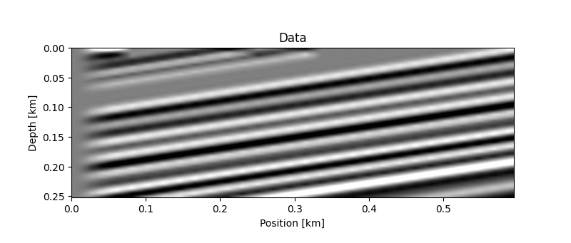
Input Data

inputfile = "../testdata/sigmoid.npz"
data = np.load(inputfile)
data = data["sigmoid"][:120, :64]
nx, nz = data.shape
dx, dz = 0.005, 0.004
x, z = np.arange(nx) * dx, np.arange(nz) * dz

aspect = dz / dx
figsize_aspect = aspect * nz / nx
opts_space = {
    "extent": (x[0], x[-1], z[-1], z[0]),
    "cmap": "gray",
    "interpolation": "lanczos",
    "aspect": aspect,
}
vmax = 0.5 * np.max(np.abs(data))
fig, ax = plt.subplots(figsize=(8, figsize_aspect * 8))
ax.imshow(data.T, vmin=-vmax, vmax=vmax, **opts_space)
ax.set(xlabel="Position [km]", ylabel="Depth [km]", title="Data")

[Text(0.5, 34.64692810457516, 'Position [km]'), Text(53.972222222222214, 0.5, 'Depth [km]'), Text(0.5, 1.0, 'Data')]

UDCT

Cop = UDCT(data.shape, num_scales=3, wedges_per_direction=3)
d_c = Cop.forward(data)

Normal Directions via FFT2D

Compute average normal vector. This vector indicates the direction normal to the structures of the image

kvecs = normal_vector_field(data, 1, 1)
kvecs *= 0.4 * min(x[-1] - x[0], z[-1] - z[0])

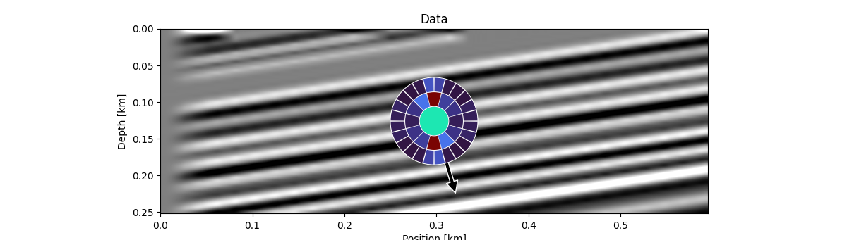
Scattering Disk via UDCT

Now we compute the average energy of each curvelet “wedge”. We will plot this on a multiscale disk to show the distribution of energies along different directions of the various scales in the data.

energy_c = apply_along_wedges(d_c, lambda w, *_: np.sqrt((np.abs(w) ** 2).mean()))

fig, ax = plt.subplots(figsize=(12, figsize_aspect * 8))
ax.imshow(data.T, vmin=-vmax, vmax=vmax, **opts_space)
overlay_arrows(kvecs, ax, arrowprops={"edgecolor": "w", "facecolor": "k"})
ax_o = create_inset_axes_grid(ax, width=0.4, kwargs_inset_axes={"projection": "polar"})
overlay_disk(energy_c, ax=ax_o, vmin=0, cmap="turbo", linecolor="w", linewidth=5)
ax.set(xlabel="Position [km]", ylabel="Depth [km]", title="Data")

[Text(0.5, 8.26888888888889, 'Position [km]'), Text(181.12037037037038, 0.5, 'Depth [km]'), Text(0.5, 1.0, 'Data')]