Meyer Wavelet Transform

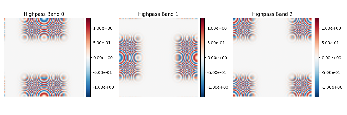
This example demonstrates the Meyer wavelet transform using a zone plate test image. The Meyer wavelet decomposes a 2D signal into 4 subbands: 1 lowpass subband and 3 highpass subbands (horizontal low-high, vertical high-low, and diagonal high-high). The transform is perfectly invertible, allowing exact reconstruction of the original signal.

# sphinx_gallery_thumbnail_number = 4

from __future__ import annotations

import matplotlib.pyplot as plt
import numpy as np
from matplotlib import ticker
from numpy.fft import fftfreq, fftshift

from curvelets.numpy import MeyerWavelet
from curvelets.plot import create_colorbar, despine
from curvelets.utils import make_zone_plate

Setup

shape = (256, 256)
zone_plate = make_zone_plate(shape)
wavelet = MeyerWavelet(shape=shape)

Meyer Wavelet Forward Transform

coefficients = wavelet.forward(zone_plate)
lowpass = coefficients[0][0]
highpass_bands = coefficients[1]

print(f"Input shape: {zone_plate.shape}")  # noqa: T201
print(f"Number of subband groups: {len(coefficients)}")  # noqa: T201
print(f"Lowpass shape: {lowpass.shape}")  # noqa: T201
print(f"Number of highpass bands: {len(highpass_bands)}")  # noqa: T201
for i, band in enumerate(highpass_bands):
    print(f"Highpass band {i} shape: {band.shape}")  # noqa: T201

Input shape: (256, 256)
Number of subband groups: 2
Lowpass shape: (128, 128)
Number of highpass bands: 3
Highpass band 0 shape: (128, 128)
Highpass band 1 shape: (128, 128)
Highpass band 2 shape: (128, 128)

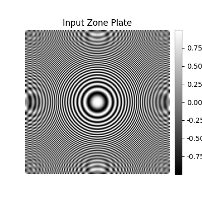
Input Image

vmax = np.abs(zone_plate).max()
opts = {"aspect": "equal", "cmap": "gray", "vmin": -vmax, "vmax": vmax}

fig, ax = plt.subplots(figsize=(4, 4))
im = ax.imshow(zone_plate.T, **opts)
_, cb = create_colorbar(im=im, ax=ax)
fmt = ticker.FuncFormatter(lambda x, _: f"{x:.2f}")
cb.ax.yaxis.set_major_formatter(fmt)
despine(ax)
ax.set(title="Input Zone Plate")

[Text(0.5, 1.0, 'Input Zone Plate')]

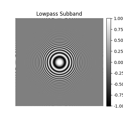
Lowpass Subband

lowpass_vmax = np.abs(lowpass).max()
lowpass_opts = {
    "aspect": "equal",
    "cmap": "gray",
    "vmin": -lowpass_vmax,
    "vmax": lowpass_vmax,
}

fig, ax = plt.subplots(figsize=(4, 4))
im = ax.imshow(lowpass.T, **lowpass_opts)
_, cb = create_colorbar(im=im, ax=ax)
fmt = ticker.FuncFormatter(lambda x, _: f"{x:.2f}")
cb.ax.yaxis.set_major_formatter(fmt)
despine(ax)
ax.set(title="Lowpass Subband")

[Text(0.5, 1.0, 'Lowpass Subband')]

Highpass Subbands

# For 2D, we have 3 highpass bands:
# - Band 0: Low-Low (after first dimension) -> High-Low (after second dimension)
# - Band 1: Low-High (after first dimension) -> Low-High (after second dimension)
# - Band 2: High-Low (after first dimension) -> High-High (after second dimension)
# Note: The exact interpretation depends on the order of dimension processing

band_names = ["Highpass Band 0", "Highpass Band 1", "Highpass Band 2"]
highpass_vmax = max(np.abs(band).max() for band in highpass_bands)
highpass_opts = {
    "aspect": "equal",
    "cmap": "RdBu_r",
    "vmin": -highpass_vmax,
    "vmax": highpass_vmax,
}

fig, axs = plt.subplots(1, 3, figsize=(12, 4))
for ax, band, name in zip(axs, highpass_bands, band_names):
    im = ax.imshow(band.T, **highpass_opts)
    _, cb = create_colorbar(im=im, ax=ax)
    fmt = ticker.FuncFormatter(lambda x, _: f"{x:.2e}")
    cb.ax.yaxis.set_major_formatter(fmt)
    despine(ax)
    ax.set(title=name)
fig.tight_layout()

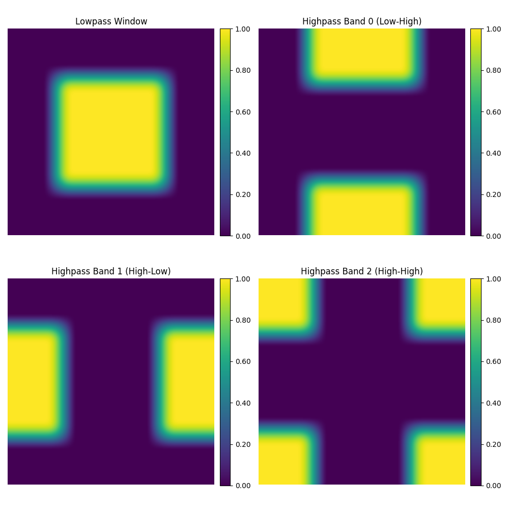
Frequency Domain Windows

Visualize the frequency domain windows (lowpass and highpass) that define the Meyer wavelet decomposition in 2D frequency space.

# Access the pre-computed 1D filters
lowpass_1d, highpass_1d = wavelet._filters[shape[0]]

# Construct 2D frequency domain windows using outer products
# For 2D Meyer wavelet, the windows are separable (product of 1D filters)
lowpass_window_2d = np.outer(lowpass_1d, lowpass_1d)
highpass_window_0_2d = np.outer(lowpass_1d, highpass_1d)  # Low-High
highpass_window_1_2d = np.outer(highpass_1d, lowpass_1d)  # High-Low
highpass_window_2_2d = np.outer(highpass_1d, highpass_1d)  # High-High

# Apply fftshift to center the frequency domain for visualization
lowpass_window_shifted = fftshift(lowpass_window_2d)
highpass_window_0_shifted = fftshift(highpass_window_0_2d)
highpass_window_1_shifted = fftshift(highpass_window_1_2d)
highpass_window_2_shifted = fftshift(highpass_window_2_2d)

# Frequency coordinates for axis labels
nx, ny = shape
kx = fftshift(fftfreq(nx))
ky = fftshift(fftfreq(ny))

# Create figure with 4 subplots
fig, axs = plt.subplots(2, 2, figsize=(10, 10))
axs = axs.flatten()

# Window names and data
window_names = [
    "Lowpass Window",
    "Highpass Band 0 (Low-High)",
    "Highpass Band 1 (High-Low)",
    "Highpass Band 2 (High-High)",
]
windows_shifted = [
    lowpass_window_shifted,
    highpass_window_0_shifted,
    highpass_window_1_shifted,
    highpass_window_2_shifted,
]

# Find common vmax for all windows
vmax = max(np.abs(w).max() for w in windows_shifted)
window_opts = {
    "aspect": "equal",
    "cmap": "viridis",
    "vmin": 0,
    "vmax": vmax,
    "extent": [kx[0], kx[-1], ky[-1], ky[0]],
}

for ax, window, name in zip(axs, windows_shifted, window_names):
    im = ax.imshow(window.T, **window_opts)
    _, cb = create_colorbar(im=im, ax=ax)
    fmt = ticker.FuncFormatter(lambda x, _: f"{x:.2f}")
    cb.ax.yaxis.set_major_formatter(fmt)
    ax.xaxis.set_minor_locator(ticker.MultipleLocator(0.1))
    ax.yaxis.set_minor_locator(ticker.MultipleLocator(0.1))
    ax.set(
        xlim=[kx[0], -kx[0]],
        ylim=[-ky[0], ky[0]],
        xlabel="Normalized $k_x$",
        ylabel="Normalized $k_y$",
        title=name,
    )
    despine(ax)
fig.tight_layout()

Energy Distribution

lowpass_energy = np.sum(np.abs(lowpass) ** 2)
highpass_energies = [np.sum(np.abs(band) ** 2) for band in highpass_bands]
total_energy = lowpass_energy + sum(highpass_energies)

print("\nEnergy Distribution:")  # noqa: T201
print(f"Lowpass: {lowpass_energy:.2e} ({100 * lowpass_energy / total_energy:.1f}%)")  # noqa: T201
for i, energy in enumerate(highpass_energies):
    print(f"Highpass {i}: {energy:.2e} ({100 * energy / total_energy:.1f}%)")  # noqa: T201
print(f"Total: {total_energy:.2e}")  # noqa: T201

Energy Distribution:
Lowpass: 2.07e+03 (25.2%)
Highpass 0: 2.05e+03 (25.0%)
Highpass 1: 2.05e+03 (25.0%)
Highpass 2: 2.03e+03 (24.7%)
Total: 8.19e+03

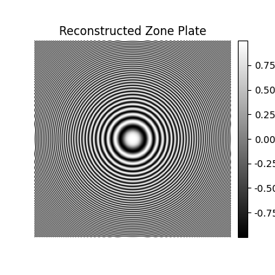
Reconstruction

reconstructed = wavelet.backward(coefficients)

Reconstructed Image

fig, ax = plt.subplots(figsize=(4, 4))
im = ax.imshow(reconstructed.T, **opts)
_, cb = create_colorbar(im=im, ax=ax)
fmt = ticker.FuncFormatter(lambda x, _: f"{x:.2f}")
cb.ax.yaxis.set_major_formatter(fmt)
despine(ax)
ax.set(title="Reconstructed Zone Plate")

[Text(0.5, 1.0, 'Reconstructed Zone Plate')]

Reconstruction Error

error = zone_plate - reconstructed
error_max = np.abs(error).max()
error_opts = {
    "aspect": "equal",
    "cmap": "RdBu_r",
    "vmin": -error_max,
    "vmax": error_max,
}

fig, ax = plt.subplots(figsize=(4, 4))
im = ax.imshow(error.T, **error_opts)
_, cb = create_colorbar(im=im, ax=ax)
fmt = ticker.FuncFormatter(lambda x, _: f"{x:.2e}")
cb.ax.yaxis.set_major_formatter(fmt)
despine(ax)
ax.set(title=f"Reconstruction Error (max = {error_max:.2e})")

print("\nReconstruction Quality:")  # noqa: T201
print(f"Max absolute error: {error_max:.2e}")  # noqa: T201
print(f"Relative error: {error_max / np.abs(zone_plate).max():.2e}")  # noqa: T201
print(f"RMSE: {np.sqrt(np.mean(error**2)):.2e}")  # noqa: T201

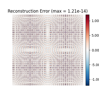
Reconstruction Quality:
Max absolute error: 1.21e-14
Relative error: 1.21e-14
RMSE: 3.62e-15