Wavelet Transforms at the Highest Scale

This example compares curvelet and wavelet transforms at the highest scale (using a simple nscale=2) on a zone plate test image. It demonstrates the difference between directional curvelet windows and a ring-shaped highpass window, showing both frequency-domain windows and spatial coefficients.

# sphinx_gallery_thumbnail_number = 2

from __future__ import annotations

import matplotlib.pyplot as plt
import numpy as np
from matplotlib import ticker
from numpy.fft import fftfreq, fftshift

from curvelets.numpy import UDCT
from curvelets.plot import create_colorbar, despine
from curvelets.utils import make_zone_plate

Setup

shape = (256, 256)
zone_plate = make_zone_plate(shape)

# Create two UDCT transforms with num_scales=2
# One in curvelet mode, one in wavelet mode
C_curvelet = UDCT(
    shape=shape,
    num_scales=2,
    wedges_per_direction=3,
    high_frequency_mode="curvelet",
)
C_wavelet = UDCT(
    shape=shape,
    num_scales=2,
    wedges_per_direction=3,
    high_frequency_mode="wavelet",
)

Forward Transforms

coeffs_curvelet = C_curvelet.forward(zone_plate)
coeffs_wavelet = C_wavelet.forward(zone_plate)

print(f"Input shape: {zone_plate.shape}")  # noqa: T201
print(f"Curvelet scales: {len(coeffs_curvelet)}")  # noqa: T201
print(f"Wavelet scales: {len(coeffs_wavelet)}")  # noqa: T201
print(f"Curvelet scale 1 directions: {len(coeffs_curvelet[1])}")  # noqa: T201
print(f"Wavelet scale 1 directions: {len(coeffs_wavelet[1])}")  # noqa: T201

Input shape: (256, 256)
Curvelet scales: 2
Wavelet scales: 2
Curvelet scale 1 directions: 2
Wavelet scale 1 directions: 1

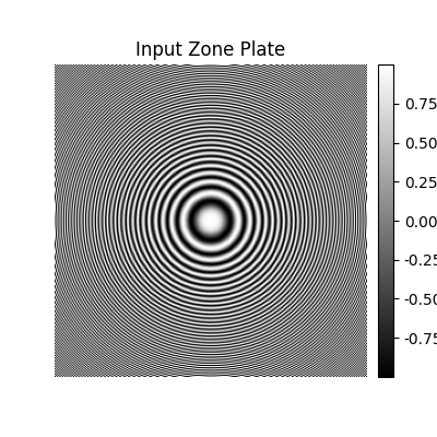
Input Image

vmax = np.abs(zone_plate).max()
opts = {"aspect": "equal", "cmap": "gray", "vmin": -vmax, "vmax": vmax}

fig, ax = plt.subplots(figsize=(4, 4))
zone_plate_real = np.real(zone_plate).astype(np.float64)
im = ax.imshow(zone_plate_real.T, **opts)
_, cb = create_colorbar(im=im, ax=ax)
fmt = ticker.FuncFormatter(lambda x, _: f"{x:.2f}")
cb.ax.yaxis.set_major_formatter(fmt)
despine(ax)
ax.set(title="Input Zone Plate")

[Text(0.5, 1.0, 'Input Zone Plate')]

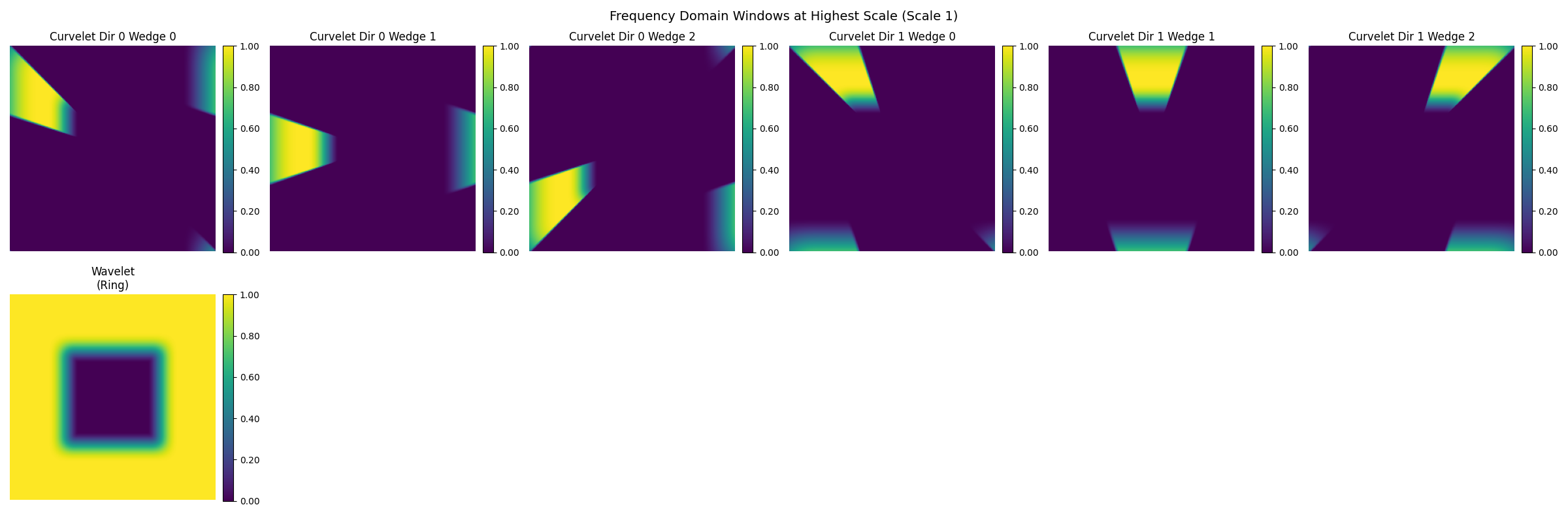
Frequency Domain Windows at Highest Scale (Scale 1)

Visualize the frequency domain windows for curvelet vs wavelet at scale 1. Curvelet windows are directional (wedges), and wavelet window is a single ring-shaped window that encompasses the entire high-frequency ring (complement of lowpass filter).

# Frequency coordinates for axis labels
nx, ny = shape
kx = fftshift(fftfreq(nx))
ky = fftshift(fftfreq(ny))

# Extract curvelet windows for scale 1
curvelet_windows_scale1 = []
curvelet_window_info = []  # Store (direction, wedge) pairs for labeling
for idir in range(len(C_curvelet.windows[1])):
    for iwedge in range(len(C_curvelet.windows[1][idir])):
        window_sparse = C_curvelet.windows[1][idir][iwedge]
        window_dense = C_curvelet._from_sparse(window_sparse)
        window_shifted = fftshift(window_dense)
        curvelet_windows_scale1.append(window_shifted)
        curvelet_window_info.append((idir, iwedge))

# Extract wavelet window for scale 1 (single ring-shaped window, complement of lowpass)
wavelet_window_sparse = C_wavelet.windows[1][0][0]
wavelet_window_dense = C_wavelet._from_sparse(wavelet_window_sparse)
wavelet_window_shifted = fftshift(wavelet_window_dense)
wavelet_windows_scale1 = [wavelet_window_shifted]

# Find common vmax for all windows
all_windows = curvelet_windows_scale1 + wavelet_windows_scale1
vmax_windows = max(np.abs(w).max() for w in all_windows)
window_opts = {
    "aspect": "equal",
    "cmap": "viridis",
    "vmin": 0,
    "vmax": vmax_windows,
    "extent": [kx[0], kx[-1], ky[-1], ky[0]],
}

# Plot curvelet and wavelet windows
n_curvelet_windows = len(curvelet_windows_scale1)
n_wavelet_windows = len(wavelet_windows_scale1)
n_cols = max(n_curvelet_windows, n_wavelet_windows)
fig, axs = plt.subplots(2, n_cols, figsize=(4 * n_cols, 8))
fig.suptitle("Frequency Domain Windows at Highest Scale (Scale 1)", fontsize=14)

# Top row: curvelet windows
for i, (window, (idir, iwedge)) in enumerate(
    zip(curvelet_windows_scale1, curvelet_window_info)
):
    ax = axs[0, i]
    window_real = np.real(window).astype(np.float64)
    im = ax.imshow(window_real.T, **window_opts)
    _, cb = create_colorbar(im=im, ax=ax)
    fmt = ticker.FuncFormatter(lambda x, _: f"{x:.2f}")
    cb.ax.yaxis.set_major_formatter(fmt)
    ax.xaxis.set_minor_locator(ticker.MultipleLocator(0.1))
    ax.yaxis.set_minor_locator(ticker.MultipleLocator(0.1))
    ax.set(
        xlim=[kx[0], -kx[0]],
        ylim=[-ky[0], ky[0]],
        xlabel="Normalized $k_x$",
        ylabel="Normalized $k_y$",
        title=f"Curvelet Dir {idir} Wedge {iwedge}",
    )
    despine(ax)

# Hide unused subplots in top row
for i in range(n_curvelet_windows, n_cols):
    axs[0, i].axis("off")

# Bottom row: wavelet window (single ring-shaped window)
wavelet_names = ["Wavelet\n(Ring)"]
for i, (window, name) in enumerate(zip(wavelet_windows_scale1, wavelet_names)):
    ax = axs[1, i]
    window_real = np.real(window).astype(np.float64)
    im = ax.imshow(window_real.T, **window_opts)
    _, cb = create_colorbar(im=im, ax=ax)
    fmt = ticker.FuncFormatter(lambda x, _: f"{x:.2f}")
    cb.ax.yaxis.set_major_formatter(fmt)
    ax.xaxis.set_minor_locator(ticker.MultipleLocator(0.1))
    ax.yaxis.set_minor_locator(ticker.MultipleLocator(0.1))
    ax.set(
        xlim=[kx[0], -kx[0]],
        ylim=[-ky[0], ky[0]],
        xlabel="Normalized $k_x$",
        ylabel="Normalized $k_y$",
        title=name,
    )
    despine(ax)

# Hide unused subplots in bottom row
for i in range(n_wavelet_windows, n_cols):
    axs[1, i].axis("off")

fig.tight_layout()

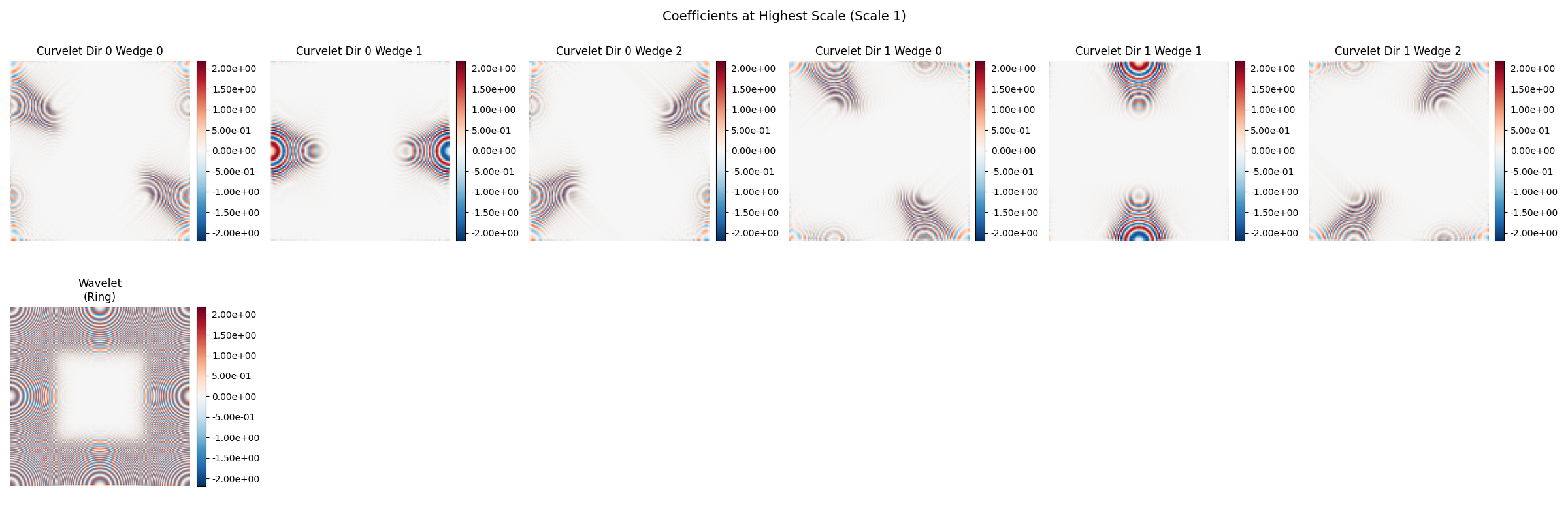
Coefficients at Highest Scale (Scale 1)

Visualize the spatial coefficients for curvelet vs wavelet at scale 1. These show how the transforms capture different features of the input.

# Extract curvelet coefficients for scale 1
curvelet_coeffs_scale1 = []
curvelet_coeff_info = []  # Store (direction, wedge) pairs for labeling
for idir in range(len(coeffs_curvelet[1])):
    for iwedge in range(len(coeffs_curvelet[1][idir])):
        coeff = coeffs_curvelet[1][idir][iwedge]
        curvelet_coeffs_scale1.append(coeff)
        curvelet_coeff_info.append((idir, iwedge))

# Extract wavelet coefficient for scale 1 (single coefficient)
wavelet_coeffs_scale1 = [coeffs_wavelet[1][0][0]]

# Find common vmax for amplitude visualization
all_coeffs = curvelet_coeffs_scale1 + wavelet_coeffs_scale1
vmax_coeffs = max(np.abs(c).max() for c in all_coeffs)
coeff_opts = {
    "aspect": "equal",
    "cmap": "RdBu_r",
    "vmin": -vmax_coeffs,
    "vmax": vmax_coeffs,
}

# Plot coefficients
n_curvelet_coeffs = len(curvelet_coeffs_scale1)
n_wavelet_coeffs = len(wavelet_coeffs_scale1)
n_cols = max(n_curvelet_coeffs, n_wavelet_coeffs)
fig, axs = plt.subplots(2, n_cols, figsize=(4 * n_cols, 8))
fig.suptitle("Coefficients at Highest Scale (Scale 1)", fontsize=14)

# Top row: curvelet coefficients
for i, (coeff, (idir, iwedge)) in enumerate(
    zip(curvelet_coeffs_scale1, curvelet_coeff_info)
):
    ax = axs[0, i]
    # Take real part for visualization (coefficients are complex but real-valued for real input)
    coeff_real = np.real(coeff).astype(np.float64)
    im = ax.imshow(coeff_real.T, **coeff_opts)
    _, cb = create_colorbar(im=im, ax=ax)
    fmt = ticker.FuncFormatter(lambda x, _: f"{x:.2e}")
    cb.ax.yaxis.set_major_formatter(fmt)
    ax.set(
        title=f"Curvelet Dir {idir} Wedge {iwedge}",
    )
    despine(ax)

# Hide unused subplots in top row
for i in range(n_curvelet_coeffs, n_cols):
    axs[0, i].axis("off")

# Bottom row: wavelet coefficient (single coefficient)
wavelet_coeff_names = ["Wavelet\n(Ring)"]
for i, (coeff, name) in enumerate(zip(wavelet_coeffs_scale1, wavelet_coeff_names)):
    ax = axs[1, i]
    # wavelet coefficient is real-valued
    coeff_real = np.real(coeff).astype(np.float64)
    im = ax.imshow(coeff_real.T, **coeff_opts)
    _, cb = create_colorbar(im=im, ax=ax)
    fmt = ticker.FuncFormatter(lambda x, _: f"{x:.2e}")
    cb.ax.yaxis.set_major_formatter(fmt)
    ax.set(title=name)
    despine(ax)

# Hide unused subplots in bottom row
for i in range(n_wavelet_coeffs, n_cols):
    axs[1, i].axis("off")

fig.tight_layout()

Summary Statistics

print("\nCurvelet Scale 1 Statistics:")  # noqa: T201
for (idir, iwedge), coeff in zip(curvelet_coeff_info, curvelet_coeffs_scale1):
    energy = np.sum(np.abs(coeff) ** 2)
    max_val = np.abs(coeff).max()
    print(  # noqa: T201
        f"  Dir {idir} Wedge {iwedge}: Energy={energy:.2e}, Max={max_val:.2e}"
    )

print("\nWavelet Scale 1 Statistics:")  # noqa: T201
for i, coeff in enumerate(wavelet_coeffs_scale1):
    energy = np.sum(np.abs(coeff) ** 2)
    max_val = np.abs(coeff).max()
    print(f"  Ring Window {i}: Energy={energy:.2e}, Max={max_val:.2e}")  # noqa: T201

Curvelet Scale 1 Statistics:
  Dir 0 Wedge 0: Energy=4.07e+03, Max=1.73e+00
  Dir 0 Wedge 1: Energy=4.10e+03, Max=2.19e+00
  Dir 0 Wedge 2: Energy=4.07e+03, Max=1.74e+00
  Dir 1 Wedge 0: Energy=4.07e+03, Max=1.73e+00
  Dir 1 Wedge 1: Energy=4.10e+03, Max=2.19e+00
  Dir 1 Wedge 2: Energy=4.07e+03, Max=1.74e+00

Wavelet Scale 1 Statistics:
  Ring Window 0: Energy=4.90e+04, Max=1.64e+00