Monogenic Curvelet Transform Verification

This example verifies the round-trip consistency of the monogenic curvelet transform by comparing the direct computation of the monogenic signal with the round-trip through the forward and backward transforms.

According to [Storath, 2010], the monogenic curvelet transform should satisfy the reproducing formula:

\[M_f(x) = \int \langle M\beta_{ab\theta}, f \rangle \cdot M\beta_{ab\theta}(x) \, db \, d\theta \, \frac{da}{a^3}\]

This means that backward(forward(f)) with transform_kind="monogenic" should produce the same result as monogenic(f), which directly computes:

\[M_f = (f, -R_1 f, -R_2 f)\]

This example verifies this property component by component, comparing:

• The scalar component with the original input f

• The Riesz_1 component with -R_1 f

• The Riesz_2 component with -R_2 f

It also includes frequency domain analysis, comparisons with the standard UDCT backward transform, and cross-term analysis to understand the reconstruction behavior.

from __future__ import annotations

from typing import Any

import matplotlib.pyplot as plt
import numpy as np
import numpy.typing as npt

from curvelets.numpy import UDCT
from curvelets.plot import create_colorbar, despine

Setup

Create a UDCT transform and a test image for verification.

shape = (256, 256)
transform = UDCT(shape=shape, num_scales=3, wedges_per_direction=3)
transform_mono = UDCT(
    shape=shape, num_scales=3, wedges_per_direction=3, transform_kind="monogenic"
)

# Create a test image (zone plate for interesting structure)
# with a window that decays to zero at the edges
x = np.linspace(-1, 1, shape[0])
y = np.linspace(-1, 1, shape[1])
X, Y = np.meshgrid(x, y, indexing="ij")
# Zone plate pattern
zone_plate = np.sin(20 * (X**2 + Y**2))
# Window function that decays to zero at all edges using Hann window
window = np.outer(np.hanning(shape[0]), np.hanning(shape[1]))
test_image = zone_plate * window

Reproducing Formula

According to Storath [2010], the monogenic curvelet transform should satisfy the reproducing formula:

\[M_f(x) = \int M_f(a,b,\theta) \cdot M_{\beta_{ab\theta}}(x) \, db \, d\theta \, \frac{da}{a^3}\]

where \(M_f(a,b,\theta) = \langle M_{\beta_{ab\theta}}, f \rangle\) are the monogenic curvelet coefficients. This means that backward(forward(f)) with transform_kind="monogenic" should produce the same result as monogenic(f), which directly computes:

\[M_f = (f, -R_1 f, -R_2 f)\]

Let’s verify this component by component.

# Method 1: Direct monogenic signal computation
scalar_direct, riesz1_direct, riesz2_direct = transform.monogenic(test_image)

# Method 2: Round-trip through monogenic curvelet transform
coeffs = transform_mono.forward(test_image)
components_round = transform_mono.backward(coeffs)
scalar_round, riesz1_round, riesz2_round = (
    components_round[0],
    components_round[1],
    components_round[2],
)

Component Comparisons

We verify the reproducing formula component by component.

f vs scalar

The scalar component should match the original input f.

fig, axs = plt.subplots(1, 4, figsize=(16, 4))

vmax = np.abs(test_image).max()
opts = {"aspect": "equal", "cmap": "RdBu_r", "vmin": -vmax, "vmax": vmax}

# Original input f
im = axs[0].imshow(test_image.T, **opts)
_, cb = create_colorbar(im=im, ax=axs[0])
despine(axs[0])
axs[0].set(title="Original input\n" + r"$f$")

# Direct: scalar_direct (should equal f)
im = axs[1].imshow(scalar_direct.T, **opts)
_, cb = create_colorbar(im=im, ax=axs[1])
despine(axs[1])
axs[1].set(title="monogenic(f)[0]")

# Round-trip: scalar_round
im = axs[2].imshow(scalar_round.T, **opts)
_, cb = create_colorbar(im=im, ax=axs[2])
despine(axs[2])
axs[2].set(title="backward(forward(f))[0]\n(scalar)")

# Difference
diff_scalar = scalar_round - test_image
vmax_diff = np.abs(diff_scalar).max()
opts_diff = {"aspect": "equal", "cmap": "RdBu_r", "vmin": -vmax_diff, "vmax": vmax_diff}
im = axs[3].imshow(diff_scalar.T, **opts_diff)
_, cb = create_colorbar(im=im, ax=axs[3])
despine(axs[3])
axs[3].set(title=f"Difference\nmax={vmax_diff:.4f}")

plt.tight_layout()

# Print statistics
print("Scalar component comparison:")  # noqa: T201
print(f"  Max diff (f vs scalar_round): {np.abs(test_image - scalar_round).max():.6e}")  # noqa: T201
print(  # noqa: T201
    f"  Ratio (scalar_round / f) at center: {scalar_round[128, 128] / test_image[128, 128]:.4f}"
)

Scalar component comparison:
  Max diff (f vs scalar_round): 4.440892e-16
  Ratio (scalar_round / f) at center: 1.0000

-R₁f vs riesz1

The riesz1 component should match -R₁f.

fig, axs = plt.subplots(1, 3, figsize=(12, 4))

vmax = np.abs(riesz1_direct).max()
opts = {"aspect": "equal", "cmap": "RdBu_r", "vmin": -vmax, "vmax": vmax}

# Direct: -R₁f
im = axs[0].imshow(riesz1_direct.T, **opts)
_, cb = create_colorbar(im=im, ax=axs[0])
despine(axs[0])
axs[0].set(title="monogenic(f)[1]\n" + r"$-R_1 f$")

# Round-trip: riesz1_round
im = axs[1].imshow(riesz1_round.T, **opts)
_, cb = create_colorbar(im=im, ax=axs[1])
despine(axs[1])
axs[1].set(title="backward(forward(f))[1]\n(riesz1)")

# Difference
diff_riesz1 = riesz1_round - riesz1_direct
vmax_diff = np.abs(diff_riesz1).max()
opts_diff = {"aspect": "equal", "cmap": "RdBu_r", "vmin": -vmax_diff, "vmax": vmax_diff}
im = axs[2].imshow(diff_riesz1.T, **opts_diff)
_, cb = create_colorbar(im=im, ax=axs[2])
despine(axs[2])
axs[2].set(title=f"Difference\nmax={vmax_diff:.4f}")

plt.tight_layout()

# Print statistics
print("\nRiesz_1 component comparison:")  # noqa: T201
print(f"  Max diff: {np.abs(riesz1_direct - riesz1_round).max():.6e}")  # noqa: T201

Riesz_1 component comparison:
  Max diff: 1.264667e-04

-R₂f vs riesz2

The riesz2 component should match -R₂f.

fig, axs = plt.subplots(1, 3, figsize=(12, 4))

vmax = np.abs(riesz2_direct).max()
opts = {"aspect": "equal", "cmap": "RdBu_r", "vmin": -vmax, "vmax": vmax}

# Direct: -R₂f
im = axs[0].imshow(riesz2_direct.T, **opts)
_, cb = create_colorbar(im=im, ax=axs[0])
despine(axs[0])
axs[0].set(title="monogenic(f)[2]\n" + r"$-R_2 f$")

# Round-trip: riesz2_round
im = axs[1].imshow(riesz2_round.T, **opts)
_, cb = create_colorbar(im=im, ax=axs[1])
despine(axs[1])
axs[1].set(title="backward(forward(f))[2]\n(riesz2)")

# Difference
diff_riesz2 = riesz2_round - riesz2_direct
vmax_diff = np.abs(diff_riesz2).max()
opts_diff = {"aspect": "equal", "cmap": "RdBu_r", "vmin": -vmax_diff, "vmax": vmax_diff}
im = axs[2].imshow(diff_riesz2.T, **opts_diff)
_, cb = create_colorbar(im=im, ax=axs[2])
despine(axs[2])
axs[2].set(title=f"Difference\nmax={vmax_diff:.4f}")

plt.tight_layout()

# Print statistics
print("\nRiesz_2 component comparison:")  # noqa: T201
print(f"  Max diff: {np.abs(riesz2_direct - riesz2_round).max():.6e}")  # noqa: T201

Riesz_2 component comparison:
  Max diff: 1.264667e-04

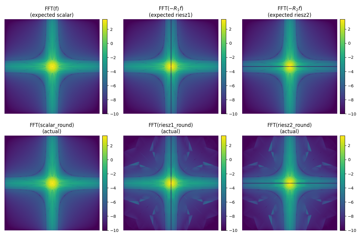
Frequency Domain Analysis

To understand the mismatch, let’s look at the frequency domain. We compare the FFT of the reconstructed components.

fig, axs = plt.subplots(2, 3, figsize=(12, 8))

# Row 1: Direct monogenic (expected)
freq_f = np.fft.fftshift(np.fft.fft2(test_image))
freq_r1_direct = np.fft.fftshift(np.fft.fft2(riesz1_direct))
freq_r2_direct = np.fft.fftshift(np.fft.fft2(riesz2_direct))

# Row 2: Round-trip (actual)
freq_scalar_round = np.fft.fftshift(np.fft.fft2(scalar_round))
freq_r1_round = np.fft.fftshift(np.fft.fft2(riesz1_round))
freq_r2_round = np.fft.fftshift(np.fft.fft2(riesz2_round))


# Plot with log scale for better visualization
def plot_freq(ax: Any, data: npt.NDArray[np.complexfloating], title: str) -> None:
    """Plot frequency magnitude on log scale."""
    mag = np.abs(data)
    mag[mag < 1e-10] = 1e-10  # Avoid log(0)
    im = ax.imshow(np.log10(mag).T, aspect="equal", cmap="viridis")
    create_colorbar(im=im, ax=ax)
    despine(ax)
    ax.set(title=title)


plot_freq(axs[0, 0], freq_f, "FFT(f)\n(expected scalar)")
plot_freq(axs[0, 1], freq_r1_direct, r"FFT($-R_1 f$)" + "\n(expected riesz1)")
plot_freq(axs[0, 2], freq_r2_direct, r"FFT($-R_2 f$)" + "\n(expected riesz2)")

plot_freq(axs[1, 0], freq_scalar_round, "FFT(scalar_round)\n(actual)")
plot_freq(axs[1, 1], freq_r1_round, "FFT(riesz1_round)\n(actual)")
plot_freq(axs[1, 2], freq_r2_round, "FFT(riesz2_round)\n(actual)")

plt.tight_layout()

Comparison with Standard UDCT Backward

The standard UDCT backward transform should perfectly reconstruct f. Let’s compare the scalar component with what standard backward gives.

# Standard UDCT round-trip
coeffs_standard = transform.forward(test_image)
recon_standard = transform.backward(coeffs_standard)

# Also try: what if we just use the scalar coefficients from monogenic
# and apply standard backward transform logic?
# Extract just the scalar coefficients (c0) from monogenic coefficients
scalar_coeffs_only = [
    [
        [coeffs[scale][dir][wedge][0] for wedge in range(len(coeffs[scale][dir]))]
        for dir in range(len(coeffs[scale]))
    ]
    for scale in range(len(coeffs))
]

# Apply standard backward to scalar-only coefficients
recon_from_scalar = transform.backward(scalar_coeffs_only)

fig, axs = plt.subplots(1, 4, figsize=(16, 4))

vmax = np.abs(test_image).max()
opts = {"aspect": "equal", "cmap": "RdBu_r", "vmin": -vmax, "vmax": vmax}

# Original
im = axs[0].imshow(test_image.T, **opts)
_, cb = create_colorbar(im=im, ax=axs[0])
despine(axs[0])
axs[0].set(title="Original f")

# Standard UDCT backward
im = axs[1].imshow(recon_standard.T, **opts)
_, cb = create_colorbar(im=im, ax=axs[1])
despine(axs[1])
diff_std = np.abs(test_image - recon_standard).max()
axs[1].set(title=f"Standard backward(forward(f))\nmax diff={diff_std:.2e}")

# Backward using only scalar coeffs from monogenic
im = axs[2].imshow(recon_from_scalar.T, **opts)
_, cb = create_colorbar(im=im, ax=axs[2])
despine(axs[2])
diff_scalar_only = np.abs(test_image - recon_from_scalar).max()
axs[2].set(title=f"backward(c₀ only)\nmax diff={diff_scalar_only:.2e}")

# Monogenic backward scalar component
im = axs[3].imshow(scalar_round.T, **opts)
_, cb = create_colorbar(im=im, ax=axs[3])
despine(axs[3])
diff_mono = np.abs(test_image - scalar_round).max()
axs[3].set(title=f"backward()[0] (monogenic)\nmax diff={diff_mono:.2e}")

plt.tight_layout()

print("\nScalar reconstruction comparison:")  # noqa: T201
print(f"  Standard backward:          max diff = {diff_std:.6e}")  # noqa: T201
print(f"  backward(c₀ only):          max diff = {diff_scalar_only:.6e}")  # noqa: T201
print(f"  backward()[0] (monogenic):  max diff = {diff_mono:.6e}")  # noqa: T201

Scalar reconstruction comparison:
  Standard backward:          max diff = 4.440892e-16
  backward(c₀ only):          max diff = 4.440892e-16
  backward()[0] (monogenic):  max diff = 4.440892e-16

Cross-term Analysis

The quaternion multiplication adds cross-terms to the scalar reconstruction: scalar = c₀·W + c₁·(W·R₁) + c₂·(W·R₂)

Let’s analyze the contribution of each term.

# For one wedge, analyze the contributions
scale_idx = 1  # First high-frequency scale
dir_idx = 0
wedge_idx = 0

c0 = coeffs[scale_idx][dir_idx][wedge_idx][0]
c1 = coeffs[scale_idx][dir_idx][wedge_idx][1]
c2 = coeffs[scale_idx][dir_idx][wedge_idx][2]

print(  # noqa: T201
    f"\nCoefficient magnitudes for scale={scale_idx}, dir={dir_idx}, wedge={wedge_idx}:"
)
print(f"  |c₀| (scalar):  max={np.abs(c0).max():.6e}, mean={np.abs(c0).mean():.6e}")  # noqa: T201
print(f"  |c₁| (riesz1):  max={np.abs(c1).max():.6e}, mean={np.abs(c1).mean():.6e}")  # noqa: T201
print(f"  |c₂| (riesz2):  max={np.abs(c2).max():.6e}, mean={np.abs(c2).mean():.6e}")  # noqa: T201

# The cross-terms c₁·(W·R₁) and c₂·(W·R₂) contribute to the scalar reconstruction
# through quaternion multiplication. When the Riesz coefficients c₁ and c₂ are
# significant relative to c₀, these cross-terms explain why backward()[0] with transform_kind="monogenic"
# may differ from the original input f even though the scalar coefficients c₀ alone
# would perfectly reconstruct f through the standard backward transform.

Coefficient magnitudes for scale=1, dir=0, wedge=0:
  |c₀| (scalar):  max=1.687700e-05, mean=1.803014e-06
  |c₁| (riesz1):  max=1.540777e-05, mean=1.079959e-06
  |c₂| (riesz2):  max=5.993421e-06, mean=3.854225e-07

Summary Statistics

print("\n" + "=" * 60)  # noqa: T201
print("SUMMARY: Component-by-Component Comparison")  # noqa: T201
print("=" * 60)  # noqa: T201
print(f"Scalar:  max|f - scalar_round| = {np.abs(test_image - scalar_round).max():.6e}")  # noqa: T201
print(  # noqa: T201
    f"Riesz1:  max|-R₁f - riesz1_round| = {np.abs(riesz1_direct - riesz1_round).max():.6e}"
)
print(  # noqa: T201
    f"Riesz2:  max|-R₂f - riesz2_round| = {np.abs(riesz2_direct - riesz2_round).max():.6e}"
)
print("=" * 60)  # noqa: T201

============================================================
SUMMARY: Component-by-Component Comparison
============================================================
Scalar:  max|f - scalar_round| = 4.440892e-16
Riesz1:  max|-R₁f - riesz1_round| = 1.264667e-04
Riesz2:  max|-R₂f - riesz2_round| = 1.264667e-04
============================================================