Monogenic Curvelet Transform

This example reproduces Figure 2 from [Storath, 2010], showing filters of usual curvelets and monogenic curvelets for an isotropic scale.

The monogenic curvelet transform extends the standard curvelet transform by applying Riesz transforms, producing three components per band that form a quaternion-like structure. This enables meaningful amplitude/phase decomposition over all scales, unlike the standard curvelet transform which only provides this decomposition at the highest scale.

Mathematical Foundation

The monogenic signal \(M_f\) of a real-valued function \(f\) is defined as:

\[M_f = f + i(-R_1f) + j(-R_2f)\]

where \(R_1\) and \(R_2\) are the first two Riesz transforms, defined in the frequency domain as:

\[\widehat{R_k(f)}(\xi) = i \frac{\xi_k}{|\xi|} \widehat{f}(\xi)\]

for \(k = 1, 2\), where \(\widehat{f}\) is the Fourier transform of \(f\), \(\xi = (\xi_1, \xi_2)\) is the frequency vector, and \(|\xi|\) is its magnitude.

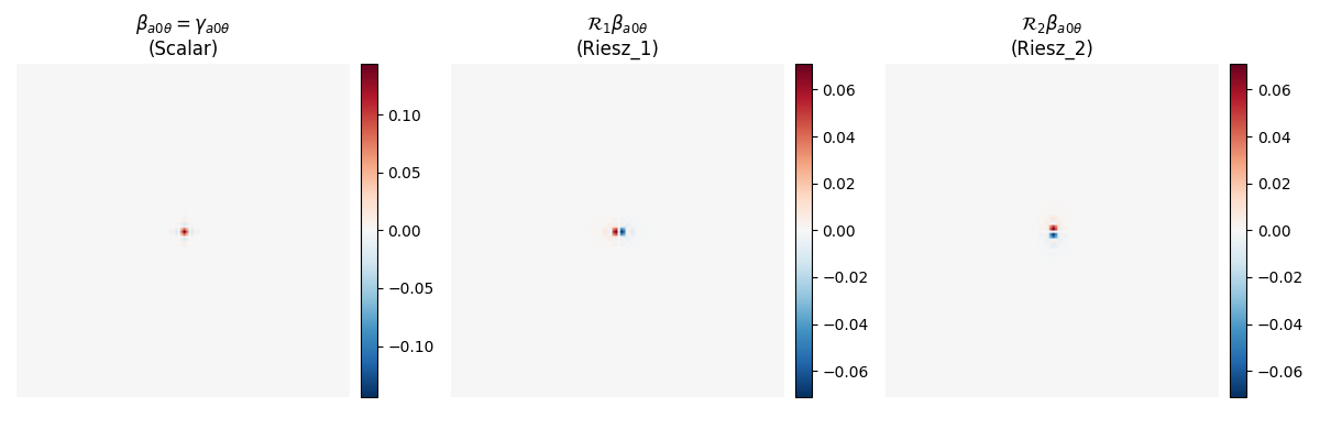
The monogenic curvelet transform applies this monogenic signal construction to each curvelet band \(\beta_{a\theta}\) (where \(a\) is scale and \(\theta\) is direction), producing three components:

• Scalar component \(\beta_{a\theta}\): Same as the standard curvelet coefficient

• Riesz_1 component \(\mathcal{R}_1\beta_{a\theta}\): First Riesz transform applied to the curvelet

• Riesz_2 component \(\mathcal{R}_2\beta_{a\theta}\): Second Riesz transform applied to the curvelet

The amplitude of the monogenic signal is computed as:

\[|M| = \sqrt{|\beta|^2 + (\mathcal{R}_1\beta)^2 + (\mathcal{R}_2\beta)^2}\]

This amplitude provides a scale-invariant measure of local structure, enabling meaningful phase/amplitude analysis at all scales.

Note

The monogenic curvelet transform was originally defined for 2D signals by [Storath, 2010] using quaternions, but this implementation extends it to arbitrary N-D signals by using all Riesz transform components (one per dimension).

from __future__ import annotations

import matplotlib.pyplot as plt
import numpy as np

from curvelets.numpy import UDCT
from curvelets.numpy._riesz import riesz_filters
from curvelets.plot import create_colorbar, despine

Setup: Create a curvelet at isotropic scale

We’ll extract the low-frequency band (isotropic scale) and visualize the scalar component and its Riesz transforms.

shape = (256, 256)
# Use smaller window overlap for better reconstruction accuracy
transform = UDCT(
    shape=shape,
    num_scales=3,
    wedges_per_direction=3,
    window_overlap=0.1,
    transform_kind="monogenic",
)

# Create a delta function at the center to visualize the curvelet
image = np.zeros(shape)
image[shape[0] // 2, shape[1] // 2] = 1.0

# Get monogenic coefficients
coeffs_mono = transform.forward(image)

# Extract the low-frequency band (scale 0, isotropic)
scalar_low = coeffs_mono[0][0][0][0]  # Scalar component
riesz1_low = coeffs_mono[0][0][0][1]  # Riesz_1 component
riesz2_low = coeffs_mono[0][0][0][2]  # Riesz_2 component

Time Domain Visualization

Figure 2a: From left to right: \(\beta_{a0\theta} = \gamma_{a0\theta}\), \(\mathcal{R}_1\beta_{a0\theta}\), and \(\mathcal{R}_2\beta_{a0\theta}\)

fig, axs = plt.subplots(1, 3, figsize=(12, 4))

# Scalar component (:math:`\beta = \gamma` at isotropic scale)
vmax = np.abs(scalar_low).max()
opts = {"aspect": "equal", "cmap": "RdBu_r", "vmin": -vmax, "vmax": vmax}

im = axs[0].imshow(np.real(scalar_low.T), **opts)
_, cb = create_colorbar(im=im, ax=axs[0])
despine(axs[0])
axs[0].set(title=r"$\beta_{a0\theta} = \gamma_{a0\theta}$" + "\n" + "(Scalar)")

# Riesz_1 component
vmax = np.abs(riesz1_low).max()
opts["vmax"] = vmax
opts["vmin"] = -vmax

im = axs[1].imshow(riesz1_low.T, **opts)
_, cb = create_colorbar(im=im, ax=axs[1])
despine(axs[1])
axs[1].set(title=r"$\mathcal{R}_1\beta_{a0\theta}$" + "\n" + "(Riesz_1)")

# Riesz_2 component
im = axs[2].imshow(riesz2_low.T, **opts)
_, cb = create_colorbar(im=im, ax=axs[2])
despine(axs[2])
axs[2].set(title=r"$\mathcal{R}_2\beta_{a0\theta}$" + "\n" + "(Riesz_2)")

plt.tight_layout()

Frequency Domain Visualization

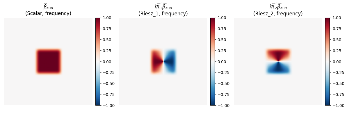
Figure 2b: From left to right: \(\widehat{\beta}_{a0\theta}\), \(i\widehat{\mathcal{R}_1\beta}_{a0\theta}\), and \(i\widehat{\mathcal{R}_2\beta}_{a0\theta}\)

To visualize in frequency domain, we compute the FFT of each component and apply the Riesz filters in frequency domain. The Riesz transforms are applied as \(i \cdot R_k \cdot \widehat{\beta}\), where \(R_k\) is the Riesz filter in frequency domain.

# Get the low-frequency window to understand the frequency support
window = transform.windows[0][0][0]
idx, val = window

# Create frequency-domain representation
frequency_band = np.zeros(shape, dtype=np.complex128)
frequency_band.flat[idx] = val

# Apply Riesz filters in frequency domain
riesz_filters_list = riesz_filters(shape)
riesz1_filter = riesz_filters_list[0]
riesz2_filter = riesz_filters_list[1]

# Frequency domain: :math:`\widehat{\beta}`
freq_scalar = frequency_band.copy()

# Frequency domain: :math:`i\widehat{\mathcal{R}_1\beta} = i \cdot R_1 \cdot \widehat{\beta}`
freq_riesz1 = 1j * riesz1_filter * frequency_band

# Frequency domain: :math:`i\widehat{\mathcal{R}_2\beta} = i \cdot R_2 \cdot \widehat{\beta}`
freq_riesz2 = 1j * riesz2_filter * frequency_band

# Visualize frequency domain
fig, axs = plt.subplots(1, 3, figsize=(12, 4))

# Shift zero frequency to center for visualization
freq_scalar_shifted = np.fft.fftshift(freq_scalar)
freq_riesz1_shifted = np.fft.fftshift(freq_riesz1)
freq_riesz2_shifted = np.fft.fftshift(freq_riesz2)

vmax = np.abs(freq_scalar_shifted).max()
opts = {"aspect": "equal", "cmap": "RdBu_r", "vmin": -vmax, "vmax": vmax}

im = axs[0].imshow(np.real(freq_scalar_shifted).T, **opts)
_, cb = create_colorbar(im=im, ax=axs[0])
despine(axs[0])
axs[0].set(title=r"$\widehat{\beta}_{a0\theta}$" + "\n" + "(Scalar, frequency)")

vmax = np.abs(freq_riesz1_shifted).max()
opts["vmax"] = vmax
opts["vmin"] = -vmax

im = axs[1].imshow(np.real(freq_riesz1_shifted).T, **opts)
_, cb = create_colorbar(im=im, ax=axs[1])
despine(axs[1])
axs[1].set(
    title=r"$i\widehat{\mathcal{R}_1\beta}_{a0\theta}$" + "\n" + "(Riesz_1, frequency)"
)

im = axs[2].imshow(np.real(freq_riesz2_shifted).T, **opts)
_, cb = create_colorbar(im=im, ax=axs[2])
despine(axs[2])
axs[2].set(
    title=r"$i\widehat{\mathcal{R}_2\beta}_{a0\theta}$" + "\n" + "(Riesz_2, frequency)"
)

plt.tight_layout()

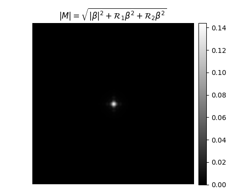
Amplitude Computation

The amplitude of the monogenic signal is computed as:

\[|M| = \sqrt{|\beta|^2 + (\mathcal{R}_1\beta)^2 + (\mathcal{R}_2\beta)^2}\]

For the scalar component, we use \(|\beta|\) since it’s complex (matching the standard curvelet transform behavior). The Riesz components are real-valued.

amplitude = np.sqrt(np.abs(scalar_low) ** 2 + riesz1_low**2 + riesz2_low**2)

fig, ax = plt.subplots(figsize=(5, 4))
vmax = amplitude.max()
opts = {"aspect": "equal", "cmap": "gray", "vmin": 0, "vmax": vmax}

im = ax.imshow(amplitude.T, **opts)
_, cb = create_colorbar(im=im, ax=ax)
despine(ax)
ax.set(title=r"$|M| = \sqrt{|\beta|^2 + \mathcal{R}_1\beta^2 + \mathcal{R}_2\beta^2}$")

plt.tight_layout()