UDCT MNIST Classification

This example demonstrates how to use UDCTModule as a feature extractor for image classification on the MNIST dataset.

Instead of using convolutional layers, this network:

1. Applies the Uniform Discrete Curvelet Transform (UDCT) to each image

2. Uses all curvelet coefficients as features (every pixel in every wedge)

3. Passes features through a two-layer MLP to classify into 10 digit classes

The key insight is that curvelet coefficients capture directional information at multiple scales, providing a meaningful representation for classification.

Architecture Overview

• Input: MNIST images (28x28 grayscale)

• Feature extraction: UDCTModule transforms each image into curvelet coefficients

• Features: All coefficient values (every pixel in every wedge) form the feature vector

• Classification: Two-layer MLP (Linear -> ReLU -> Linear) maps features to 10 classes

• Batch processing: torch.vmap enables efficient batched inference

Credits

This example is adapted from the PyTorch MNIST example.

# sphinx_gallery_thumbnail_number = 2

from __future__ import annotations

import matplotlib.pyplot as plt
import torch
import torch.nn.functional as F
from sklearn.manifold import TSNE
from torch import nn, optim
from torch.optim.lr_scheduler import StepLR
from torchvision import datasets, transforms

from curvelets.torch import UDCTModule

UDCTNet: Curvelet-Based Classifier

This network replaces convolutional layers with the curvelet transform. The key components are:

1. UDCTModule: Computes curvelet coefficients for each image

2. Feature extraction: Uses all coefficient values as features

3. Two-layer MLP: Maps features to class probabilities

We use torch.vmap to efficiently process batches of images.

class UDCTNet(nn.Module):  # type: ignore[misc]
    """Neural network using UDCT for feature extraction."""

    def __init__(
        self,
        shape: tuple[int, int] = (28, 28),
        num_scales: int = 2,
        wedges_per_direction: int = 3,
        hidden_size: int = 128,
    ) -> None:
        super().__init__()
        self.udct = UDCTModule(
            shape=shape,
            num_scales=num_scales,
            wedges_per_direction=wedges_per_direction,
        )
        # Precompute number of features via dummy forward pass during init
        # UDCTModule returns flattened coefficients (all pixels in all wedges)
        with torch.inference_mode():
            dummy = torch.zeros(shape)
            n_features = self.udct(dummy).numel()
        self.fc1 = nn.Linear(n_features, hidden_size)
        self.fc2 = nn.Linear(hidden_size, 10)

    def _extract_features(self, x: torch.Tensor) -> torch.Tensor:
        """Extract all curvelet coefficients from a single 2D image."""
        # UDCTModule returns flattened coefficients - take abs to get real features
        return self.udct(x).abs()

    def forward(self, x: torch.Tensor) -> torch.Tensor:
        """Forward pass with batched curvelet feature extraction."""
        # x: (batch, 1, 28, 28) -> squeeze to (batch, 28, 28)
        x = x.squeeze(1)
        # Use vmap for batch processing
        features = torch.vmap(self._extract_features)(x)
        x = F.relu(self.fc1(features))
        return F.log_softmax(self.fc2(x), dim=1)

    def get_features(self, x: torch.Tensor) -> torch.Tensor:
        """Extract features without classification (for visualization)."""
        x = x.squeeze(1)
        return torch.vmap(self._extract_features)(x)

Training and Testing Functions

Standard PyTorch training loop with negative log-likelihood loss.

def train(
    model: nn.Module,
    device: torch.device,
    train_loader: torch.utils.data.DataLoader,
    optimizer: optim.Optimizer,
) -> tuple[float, float]:
    """Train the model for one epoch and return average loss and accuracy."""
    model.train()
    total_loss = 0.0
    correct = 0
    for _, (data, target) in enumerate(train_loader):
        data_device = data.to(device)
        target_device = target.to(device)
        optimizer.zero_grad()
        output = model(data_device)
        loss = F.nll_loss(output, target_device)
        loss.backward()
        optimizer.step()
        total_loss += loss.item()
        pred = output.argmax(dim=1, keepdim=True)
        correct += pred.eq(target_device.view_as(pred)).sum().item()
    avg_loss = total_loss / len(train_loader)
    accuracy = 100.0 * correct / len(train_loader.dataset)
    return avg_loss, accuracy


def test(
    model: nn.Module,
    device: torch.device,
    test_loader: torch.utils.data.DataLoader,
) -> tuple[float, float]:
    """Evaluate the model on the test set and return average loss and accuracy."""
    model.eval()
    test_loss = 0.0
    correct = 0
    with torch.inference_mode():
        for data, target in test_loader:
            data_device = data.to(device)
            target_device = target.to(device)
            output = model(data_device)
            test_loss += F.nll_loss(output, target_device, reduction="sum").item()
            pred = output.argmax(dim=1, keepdim=True)
            correct += pred.eq(target_device.view_as(pred)).sum().item()

    test_loss /= len(test_loader.dataset)
    accuracy = 100.0 * correct / len(test_loader.dataset)
    return test_loss, accuracy


def collect_worst_loss_misclassifications(
    model: nn.Module,
    device: torch.device,
    test_loader: torch.utils.data.DataLoader,
) -> dict[int, tuple[torch.Tensor, int, int, float]]:
    """Collect worst loss misclassified examples grouped by ground truth digit.

    For each digit class (0-9), finds the misclassified example with the
    highest loss value.

    Parameters
    ----------
    model : nn.Module
        Trained model to evaluate.
    device : torch.device
        Device to run inference on.
    test_loader : torch.utils.data.DataLoader
        DataLoader for test dataset.

    Returns
    -------
    dict[int, tuple[torch.Tensor, int, int, float]]
        Dictionary mapping ground truth digit (0-9) to a tuple of
        (image tensor, ground truth label, predicted label, loss value).
        Only contains digits that have misclassifications.
    """
    model.eval()
    worst_misclassifications: dict[int, tuple[torch.Tensor, int, int, float]] = {}

    with torch.inference_mode():
        for data, target in test_loader:
            data_device = data.to(device)
            target_device = target.to(device)
            output = model(data_device)
            pred = output.argmax(dim=1)

            # Compute loss for each sample
            # F.nll_loss with reduction='none' gives per-sample losses
            per_sample_loss = F.nll_loss(output, target_device, reduction="none")

            # Find misclassifications
            incorrect_mask = pred != target_device
            incorrect_indices = incorrect_mask.nonzero(as_tuple=True)[0]

            for idx in incorrect_indices:
                true_label = int(target_device[idx].item())
                pred_label = int(pred[idx].item())
                loss_value = float(per_sample_loss[idx].item())

                # Store worst loss example for each digit class
                if true_label not in worst_misclassifications:
                    worst_misclassifications[true_label] = (
                        data[idx].cpu(),
                        true_label,
                        pred_label,
                        loss_value,
                    )
                else:
                    # Update if this example has higher loss
                    _, _, _, current_loss = worst_misclassifications[true_label]
                    if loss_value > current_loss:
                        worst_misclassifications[true_label] = (
                            data[idx].cpu(),
                            true_label,
                            pred_label,
                            loss_value,
                        )

            # Stop if we have examples for all 10 digits
            if len(worst_misclassifications) == 10:
                break

    return worst_misclassifications

Main Training Script

We use a simplified configuration suitable for a gallery example:

• 10 epochs

• Batch size of 64

• Adadelta optimizer with learning rate scheduling

# Device selection
if torch.accelerator.is_available():
    device = torch.accelerator.current_accelerator()
else:
    device = torch.device("cpu")

# Data loading
transform = transforms.Compose(
    [transforms.ToTensor(), transforms.Normalize((0.1307,), (0.3081,))]
)

train_dataset = datasets.MNIST("./data", train=True, download=True, transform=transform)
test_dataset = datasets.MNIST("./data", train=False, transform=transform)

train_loader = torch.utils.data.DataLoader(train_dataset, batch_size=64, shuffle=True)
test_loader = torch.utils.data.DataLoader(test_dataset, batch_size=1000)

0.3%
0.7%
1.0%
1.3%
1.7%
2.0%
2.3%
2.6%
3.0%
3.3%
3.6%
4.0%
4.3%
4.6%
5.0%
5.3%
5.6%
6.0%
6.3%
6.6%
6.9%
7.3%
7.6%
7.9%
8.3%
8.6%
8.9%
9.3%
9.6%
9.9%
10.2%
10.6%
10.9%
11.2%
11.6%
11.9%
12.2%
12.6%
12.9%
13.2%
13.6%
13.9%
14.2%
14.5%
14.9%
15.2%
15.5%
15.9%
16.2%
16.5%
16.9%
17.2%
17.5%
17.9%
18.2%
18.5%
18.8%
19.2%
19.5%
19.8%
20.2%
20.5%
20.8%
21.2%
21.5%
21.8%
22.1%
22.5%
22.8%
23.1%
23.5%
23.8%
24.1%
24.5%
24.8%
25.1%
25.5%
25.8%
26.1%
26.4%
26.8%
27.1%
27.4%
27.8%
28.1%
28.4%
28.8%
29.1%
29.4%
29.8%
30.1%
30.4%
30.7%
31.1%
31.4%
31.7%
32.1%
32.4%
32.7%
33.1%
33.4%
33.7%
34.0%
34.4%
34.7%
35.0%
35.4%
35.7%
36.0%
36.4%
36.7%
37.0%
37.4%
37.7%
38.0%
38.3%
38.7%
39.0%
39.3%
39.7%
40.0%
40.3%
40.7%
41.0%
41.3%
41.7%
42.0%
42.3%
42.6%
43.0%
43.3%
43.6%
44.0%
44.3%
44.6%
45.0%
45.3%
45.6%
45.9%
46.3%
46.6%
46.9%
47.3%
47.6%
47.9%
48.3%
48.6%
48.9%
49.3%
49.6%
49.9%
50.2%
50.6%
50.9%
51.2%
51.6%
51.9%
52.2%
52.6%
52.9%
53.2%
53.6%
53.9%
54.2%
54.5%
54.9%
55.2%
55.5%
55.9%
56.2%
56.5%
56.9%
57.2%
57.5%
57.9%
58.2%
58.5%
58.8%
59.2%
59.5%
59.8%
60.2%
60.5%
60.8%
61.2%
61.5%
61.8%
62.1%
62.5%
62.8%
63.1%
63.5%
63.8%
64.1%
64.5%
64.8%
65.1%
65.5%
65.8%
66.1%
66.4%
66.8%
67.1%
67.4%
67.8%
68.1%
68.4%
68.8%
69.1%
69.4%
69.8%
70.1%
70.4%
70.7%
71.1%
71.4%
71.7%
72.1%
72.4%
72.7%
73.1%
73.4%
73.7%
74.0%
74.4%
74.7%
75.0%
75.4%
75.7%
76.0%
76.4%
76.7%
77.0%
77.4%
77.7%
78.0%
78.3%
78.7%
79.0%
79.3%
79.7%
80.0%
80.3%
80.7%
81.0%
81.3%
81.7%
82.0%
82.3%
82.6%
83.0%
83.3%
83.6%
84.0%
84.3%
84.6%
85.0%
85.3%
85.6%
85.9%
86.3%
86.6%
86.9%
87.3%
87.6%
87.9%
88.3%
88.6%
88.9%
89.3%
89.6%
89.9%
90.2%
90.6%
90.9%
91.2%
91.6%
91.9%
92.2%
92.6%
92.9%
93.2%
93.6%
93.9%
94.2%
94.5%
94.9%
95.2%
95.5%
95.9%
96.2%
96.5%
96.9%
97.2%
97.5%
97.9%
98.2%
98.5%
98.8%
99.2%
99.5%
99.8%
100.0%

100.0%

2.0%
4.0%
6.0%
7.9%
9.9%
11.9%
13.9%
15.9%
17.9%
19.9%
21.9%
23.8%
25.8%
27.8%
29.8%
31.8%
33.8%
35.8%
37.8%
39.7%
41.7%
43.7%
45.7%
47.7%
49.7%
51.7%
53.7%
55.6%
57.6%
59.6%
61.6%
63.6%
65.6%
67.6%
69.6%
71.5%
73.5%
75.5%
77.5%
79.5%
81.5%
83.5%
85.5%
87.4%
89.4%
91.4%
93.4%
95.4%
97.4%
99.4%
100.0%

100.0%

Model Initialization

Create the UDCTNet model with 2 scales and 3 wedges per direction. With all curvelet coefficients as features, we get a high-dimensional feature vector that preserves all transform information.

model = UDCTNet(shape=(28, 28), num_scales=2, wedges_per_direction=3).to(device)

Training Loop

Train for 10 epochs with Adadelta optimizer and step learning rate decay.

optimizer = optim.Adadelta(model.parameters(), lr=1.0)
scheduler = StepLR(optimizer, step_size=1, gamma=0.7)

num_epochs = 10
train_losses: list[float] = []
test_losses: list[float] = []
train_accuracies: list[float] = []
test_accuracies: list[float] = []

for _ in range(1, num_epochs + 1):
    train_loss, train_acc = train(model, device, train_loader, optimizer)
    test_loss, test_acc = test(model, device, test_loader)
    train_losses.append(train_loss)
    test_losses.append(test_loss)
    train_accuracies.append(train_acc)
    test_accuracies.append(test_acc)
    scheduler.step()

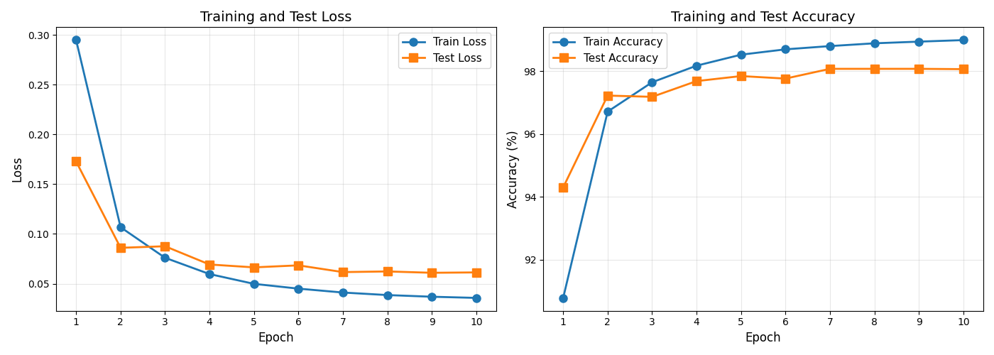
Loss and Accuracy Plot

Visualize the training and test loss and accuracy over epochs.

epochs = range(1, num_epochs + 1)

fig, (ax1, ax2) = plt.subplots(1, 2, figsize=(14, 5))

# Loss subplot
ax1.plot(epochs, train_losses, "o-", label="Train Loss", linewidth=2, markersize=8)
ax1.plot(epochs, test_losses, "s-", label="Test Loss", linewidth=2, markersize=8)
ax1.set_xlabel("Epoch", fontsize=12)
ax1.set_ylabel("Loss", fontsize=12)
ax1.set_title("Training and Test Loss", fontsize=14)
ax1.legend(fontsize=11)
ax1.grid(True, alpha=0.3)
ax1.set_xticks(epochs)

# Accuracy subplot
ax2.plot(
    epochs, train_accuracies, "o-", label="Train Accuracy", linewidth=2, markersize=8
)
ax2.plot(
    epochs, test_accuracies, "s-", label="Test Accuracy", linewidth=2, markersize=8
)
ax2.set_xlabel("Epoch", fontsize=12)
ax2.set_ylabel("Accuracy (%)", fontsize=12)
ax2.set_title("Training and Test Accuracy", fontsize=14)
ax2.legend(fontsize=11)
ax2.grid(True, alpha=0.3)
ax2.set_xticks(epochs)

plt.tight_layout()
plt.show()

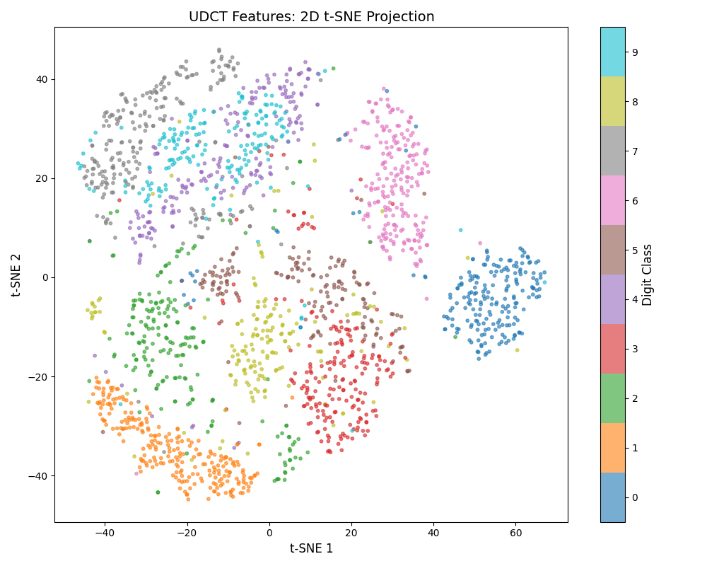
t-SNE Feature Visualization

Visualize the curvelet features in 2D using t-SNE. Each digit class is shown in a different color, revealing how well the features separate the classes.

t-SNE (t-distributed Stochastic Neighbor Embedding) is a nonlinear dimensionality reduction technique that preserves local structure.

# Extract features from a subset of training data for visualization
n_samples = 2000
subset_loader = torch.utils.data.DataLoader(
    train_dataset, batch_size=n_samples, shuffle=True
)
data_batch, labels_batch = next(iter(subset_loader))

# Extract features using the trained model
model.eval()
with torch.inference_mode():
    features_batch = model.get_features(data_batch.to(device)).cpu().numpy()
labels_np = labels_batch.numpy()

# Apply t-SNE to reduce to 2 dimensions
tsne = TSNE(n_components=2, random_state=42, perplexity=30)
features_tsne = tsne.fit_transform(features_batch)

fig, ax = plt.subplots(figsize=(10, 8))
scatter = ax.scatter(
    features_tsne[:, 0],
    features_tsne[:, 1],
    c=labels_np,
    cmap="tab10",
    vmin=-0.5,
    vmax=9.5,
    alpha=0.6,
    s=10,
)
cbar = plt.colorbar(scatter, ax=ax, ticks=range(10))
cbar.set_label("Digit Class", fontsize=12)
ax.set_xlabel("t-SNE 1", fontsize=12)
ax.set_ylabel("t-SNE 2", fontsize=12)
ax.set_title("UDCT Features: 2D t-SNE Projection", fontsize=14)
plt.tight_layout()
plt.show()

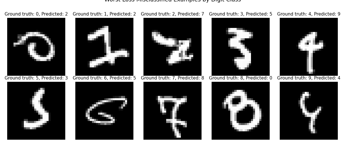
Misclassification Visualization

Display the worst loss misclassified example for each digit class (0-9) in a 2x5 grid. Each subplot shows the image with a title indicating the ground truth digit and the predicted digit. For each digit, the example with the highest loss is shown.

# Collect worst loss misclassifications from test set
worst_misclassifications = collect_worst_loss_misclassifications(
    model, device, test_loader
)

fig, axes = plt.subplots(2, 5, figsize=(12, 5))
axes = axes.flatten()

# Denormalization parameters (reverse of Normalize((0.1307,), (0.3081,)))
mean = 0.1307
std = 0.3081

for digit in range(10):
    ax = axes[digit]
    if digit in worst_misclassifications:
        img, true_label, pred_label, loss_value = worst_misclassifications[digit]
        # Denormalize image for display
        img_denorm = img.squeeze(0) * std + mean
        # Clamp to [0, 1] range
        img_denorm = torch.clamp(img_denorm, 0, 1)
        ax.imshow(img_denorm.numpy(), cmap="gray")
        ax.set_title(
            f"Ground truth: {true_label}, Predicted: {pred_label}", fontsize=11
        )
    else:
        # Handle case where digit has no misclassifications
        ax.text(
            0.5,
            0.5,
            f"No misclassifications\nfor digit {digit}",
            ha="center",
            va="center",
            transform=ax.transAxes,
            fontsize=10,
        )
        ax.set_title(f"Digit {digit}", fontsize=11)
    ax.axis("off")

plt.suptitle("Worst Loss Misclassified Examples by Digit Class", fontsize=14, y=1.02)
plt.tight_layout()
plt.show()